
Comparing power of statistical tests
Published:
As a graduate student and a postdoc, I often saw scientists deflated by statistics. All their delicate thinking and theorizing and all their very careful and painstaking experimentation has to, at some point, be subject to statistics, and the most commonly-used statistical tests simply ask, “Is this group of numbers bigger or smaller than that other group?”
To give a sense of one part of the tradeoffs in choosing a statistical test, I cooked up this very simple, and very abstract, example. Imagine you have two populations (e.g., experimental groups) with an equal number of samples in both. Further imagine that these 2 populations are normally distributed and have the same variance. The difference between the two populations is then the effect size d, which is the difference in the means divided by the (common) standard deviation.
Knowing that the populations are normally distribution, a t-test is the approach I would use. But what if you weren’t sure of the t-test, and wanted to do something simpler and more robust?
One alternative would be to divide the data into 2 groups: those points above the median of all the data, and those below. You expect that more of the population 1 points are below the median and more of the population 2 points are above the median. You can do a simple test of proportions, seeing if the proportion of population 1 points that are below the median is greater than the proportion of population 2 points below the median.
For large d, almost all the population 1 points are below the median, but for smaller d, the picture becomes muddier.
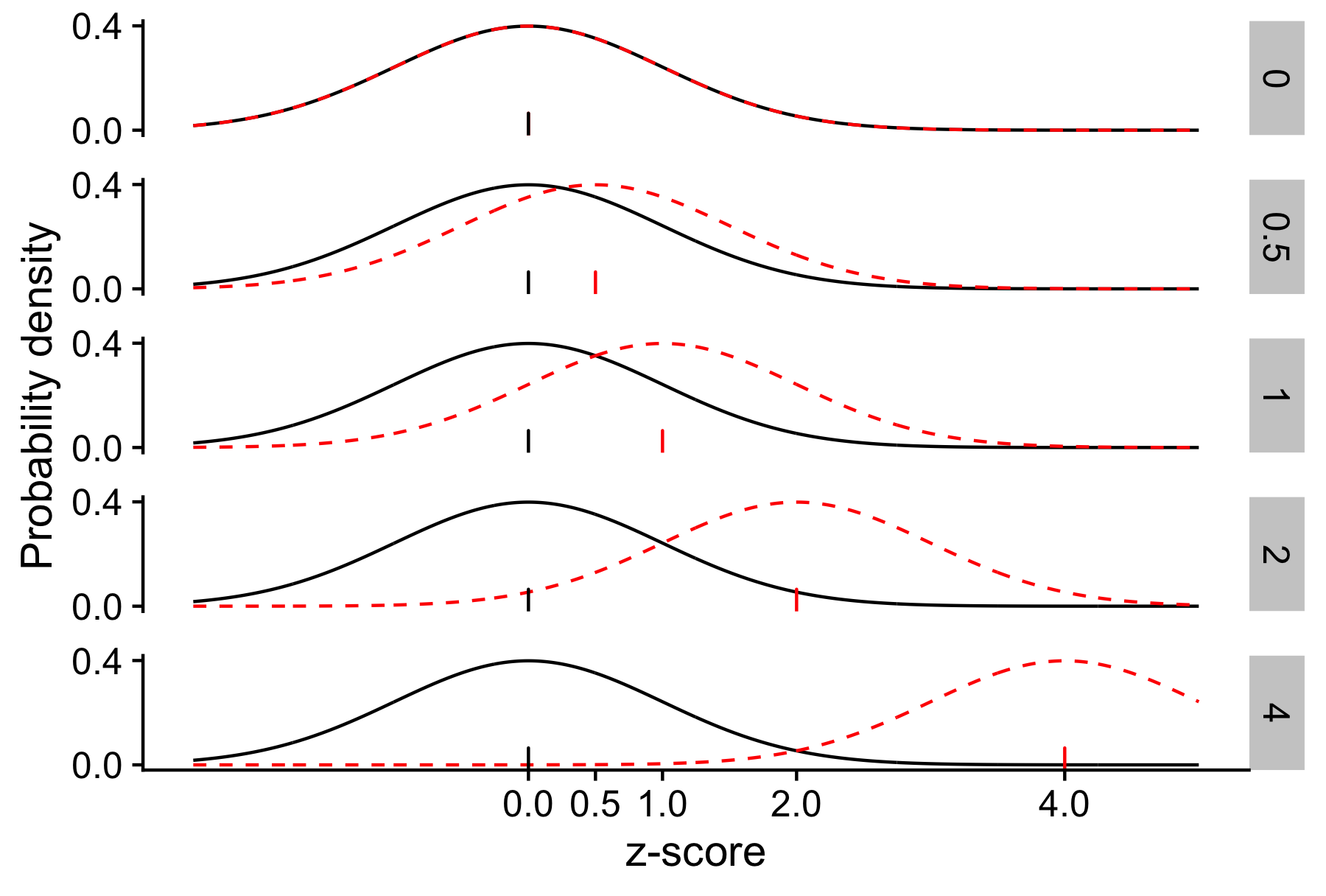
For larger effect sizes, the 2 populations have less overlap. Black lines show population 1. Dotted red lines show population 2. Ticks show the mean of each distribution. Rows show values of the effect size d.
In this example, we can directly quantify the number of samples required to get a statistically significant test with 80% probability, as a function of d:
library(tidyverse)
library(pwr)

# Given d, how many samples are needed per group to achieve 80% power
# in a t-test?
power_t_test <- function(d) pwr.t.test(d = d, power = 0.8)$n

# And for the proportion test described above?
power_prop_test <- function(d) {
  # Compute the ideal proportion of pop 1 samples below the median, which
  # is 1 minus the proportion of pop 2 samples below the median
  q <- pnorm(d / 2)
  # Compute the power calculation effect size
  h <- ES.h(q, 1 - q)
  pwr.2p.test(h = h, power = 0.8)$n
}

# Effect sizes to consider
ds <- c(0.1, 0.5, 1.0, 2.0, 4.0)

tibble(d = ds) %>%
  mutate(
    true_prop = pnorm(d / 2),
    false_prop = 1 - true_prop,
    n_t = map_dbl(d, power_t_test),
    n_prop = map_dbl(d, power_prop_test),
    fold = n_prop / n_t
  )
In the table, the “true” proportion is the number of population 1 samples below the median (and the number of population 2 samples above the median); the “false” proportion is the proportion of population 1 samples above the median, the numbers are the number of samples needed to achieve 80% statistical power under the 2 tests, and the fold difference shows how many more samples the proportion test needs to achieve the same statistical power.
| d | “True” prop. | “False” prop. | No. (t-test) | No. (prop. test) | Fold diff. |
|---|---|---|---|---|---|
| 0.1 | 0.52 | 0.480 | 1600.0 | 2500.0 | 1.6 |
| 0.5 | 0.60 | 0.400 | 64.0 | 99.0 | 1.6 |
| 1.0 | 0.69 | 0.310 | 17.0 | 25.0 | 1.5 |
| 2.0 | 0.84 | 0.160 | 5.1 | 7.0 | 1.4 |
| 4.0 | 0.98 | 0.023 | 2.4 | 2.4 | 1.0 |
As d increases, the 2 populations’ overlap declines, and the number of samples needed to detect that the populations are different declines. The t-test always outperforms the proportion test, but that difference in performance declines with d. Perhaps surprisingly, when d is large enough, it doesn’t matter which approach you use!