
purrr for analysis in R
Published:
In my postdoc work, I was running a lot of models on data. I found R really useful to doing the models, but I often struggled to write nice code around running many models. Until I discovered purrr.
As an example, say I wanted to do some analysis on the “iris” data set, which “gives the measurements in centimeters of the variables sepal length and width and petal length and width, respectively, for 50 flowers from each of 3 species of iris”, Iris setosa, I. versicolor, and I. virginica. Here are the first 3 rows:
| Sepal.Length | Sepal.Width | Petal.Length | Petal.Width | Species |
|---|---|---|---|---|
| 5.1 | 3.5 | 1.4 | 0.2 | setosa |
| 4.9 | 3.0 | 1.4 | 0.2 | setosa |
| 4.7 | 3.2 | 1.3 | 0.2 | setosa |
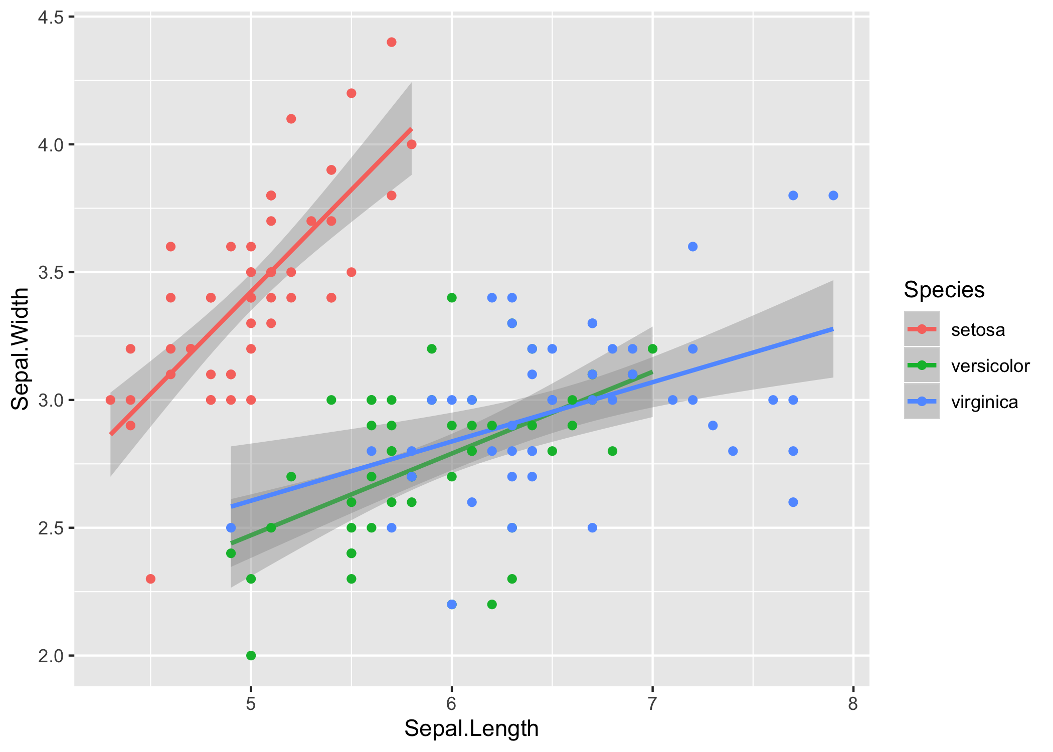
Let’s consider the relationship between sepal length and width in the three species.
library(tidyverse)
library(ggplot2)

iris %>%
  ggplot(aes(x = Sepal.Length, y = Sepal.Width, color = Species)) +
  stat_smooth(method = 'lm') +
  geom_point()
In base R it is relatively straightforward to extract the slope $m$ and intercept $b$ for a least-squares best fit to each species by specifying a model that includes interactions between species $s$ and slope. In R syntax, the least squares model \(\begin{equation} y_i = m_{s_i} x_i + b_{s_i} + \varepsilon_i \end{equation}\) is represented:
lm(Sepal.Width ~ Species * Sepal.Length, data = iris)
Running summary on that model gives the output:
Call:
lm(formula = Sepal.Width ~ Species * Sepal.Length, data = iris)

Residuals:
     Min       1Q   Median       3Q      Max
-0.72394 -0.16327 -0.00289  0.16457  0.60954

Coefficients:
                               Estimate Std. Error t value Pr(>|t|)
(Intercept)                     -0.5694     0.5539  -1.028 0.305622
Speciesversicolor                1.4416     0.7130   2.022 0.045056 *
Speciesvirginica                 2.0157     0.6861   2.938 0.003848 **
Sepal.Length                     0.7985     0.1104   7.235 2.55e-11 ***
Speciesversicolor:Sepal.Length  -0.4788     0.1337  -3.582 0.000465 ***
Speciesvirginica:Sepal.Length   -0.5666     0.1262  -4.490 1.45e-05 ***
---
Signif. codes:  0 ‘***’ 0.001 ‘**’ 0.01 ‘*’ 0.05 ‘.’ 0.1 ‘ ’ 1

Residual standard error: 0.2723 on 144 degrees of freedom
Multiple R-squared:  0.6227,	Adjusted R-squared:  0.6096
F-statistic: 47.53 on 5 and 144 DF,  p-value: < 2.2e-16
In that regression, R treated I. setosa as the “base” species, so
(Intercept) and Sepal.Length are the intercept and slope for I. setosa.
The intercept for I. versicolor is the (Intercept) term plus the
Speciesversicolor term, and the slope is the Sepal.Length term plus the
Speciesversicolor:Sepal.Length term.
This is a bit of a mess if I just wanted to know what the slopes and intercepts were for each species. If I wanted three separate models, there’s a few ways to do it.
I’ll start with the ugly, naive way, which is to make three different data frame and three different models:
# these two lines would be repeated for I. versicolor and I. virginica
setosa_data <- iris[iris$Species == 'setosa', ]
setosa_model <- lm(Sepal.Width ~ Sepal.Length, data = setosa_data)

# the slope for I. setosa
coef(setosa_model)['Sepal.Length']

# output:
# Sepal.Length
# 0.7985283
This approach, although it works for the iris data, doesn’t scale well, since
it requires a lot of manual typing of the species names. The second approach is
to use some the base R functions split, which will break the data into a list
of three separate data sets, and lapply, which will run a function on each
member of that list:
species_datasets <- split(iris, iris$Species)
species_models <- lapply(species_datasets, function(data) {
  lm(Sepal.Width ~ Sepal.Length, data = data)
})

# get the slope from the first model, which is for I. setosa
coef(species_models[[1]])['Sepal.Length']
This approach is still awkward because the data and the models are in separate objects. You need to manually keep track of them, make sure they are in the same order, etc. It would be a lot nicer if the data, the models, and whatever else you wanted to pull out from either of those were in one structure.
It turns out that, in a tibble (“a modern re-imagining of the data.frame” as per the reference docs), the columns can be lists. So one column could be a vector of string objects, the species names, and the second can be a list of models:
tibble(
  species = levels(iris$Species),
  model = species_models
)

# output:
#  # A tibble: 3 x 2
#   species    model
#   <chr>      <list>
# 1 setosa     <lm>
# 2 versicolor <lm>
# 3 virginica  <lm>
This is where purrr comes in. First, there is a function nest. Like
split, it breaks a dataset down into smaller parts. Unlike split, it keeps
them in a nice dataframe. It’s called “nest” because one of the columns in the
tibble is itself a list of the smaller tibbles.
# "minus" means put all columns except Species into the nested dataframes
nest(iris, -Species)

# output:
# # A tibble: 3 x 2
#   Species    data
#   <fct>      <list>
# 1 setosa     <tibble [50 × 4]>
# 2 versicolor <tibble [50 × 4]>
# 3 virginica  <tibble [50 × 4]>
Next, there is a family of functions map. Just like map functions in other
languages and the Map and lapply functions in base R, it takes a function
and a vector of inputs, or multiple inputs, and returns the outputs.
iris %>%
  nest(-Species) %>%
  mutate(
    # this works
    model1 = lapply(data, function(x) lm(Sepal.Width ~ Sepal.Length, data = x)),
    # "map" also works
    model2 = map(data, function(x) lm(Sepal.Width ~ Sepal.Length, data = x)),
    # "map" also allows a shorthand for anonymous functions
    model3 = map(data, ~ lm(Sepal.Width ~ Sepal.Length, data = .))
  )

# output:
# # A tibble: 3 x 5
#   Species    data              model1 model2 model3
#   <fct>      <list>            <list> <list> <list>
# 1 setosa     <tibble [50 × 4]> <lm>   <lm>   <lm>
# 2 versicolor <tibble [50 × 4]> <lm>   <lm>   <lm>
# 3 virginica  <tibble [50 × 4]> <lm>   <lm>   <lm>
The really nice bit about map is that is has close cousins like map_dbl
which specify that the output should be a vector of numbers, rather than a list
of numbers. Here’s what I mean:
iris %>%
  nest(-Species) %>%
  mutate(
    model = map(data, ~ lm(Sepal.Width ~ Sepal.Length, data = .)),
    slope1 = map(model, ~ coef(.)['Sepal.Length']),
    slope2 = map_dbl(model, ~ coef(.)['Sepal.Length'])
  )

# output:
# # A tibble: 3 x 5
#   Species    data              model  slope1    slope2
#   <fct>      <list>            <list> <list>     <dbl>
# 1 setosa     <tibble [50 × 4]> <lm>   <dbl [1]>  0.799
# 2 versicolor <tibble [50 × 4]> <lm>   <dbl [1]>  0.320
# 3 virginica  <tibble [50 × 4]> <lm>   <dbl [1]>  0.232
Note that the map for slope in the above gave a list of single numbers,
where each item in the list is a numeric vector with a single entry, while
map_dbl gave one vector that “lays” the values more nicely in the tibble.
Now it’s nice and easy to compare the models in the context of a data frame:
iris %>%
  nest(-Species) %>%
  mutate(
    model = map(data, ~ lm(Sepal.Width ~ Sepal.Length, data = .)),
    slope = map_dbl(model, ~ coef(.)['Sepal.Length']),
    slope_confint = map(model, ~ confint(.)['Sepal.Length', ]),
    slope_cil = map_dbl(slope_confint, first),
    slope_ciu = map_dbl(slope_confint, last)
  ) %>%
  ggplot(aes(x = Species, y = slope, ymin = slope_cil, ymax = slope_ciu)) +
  geom_point() +
  geom_errorbar()
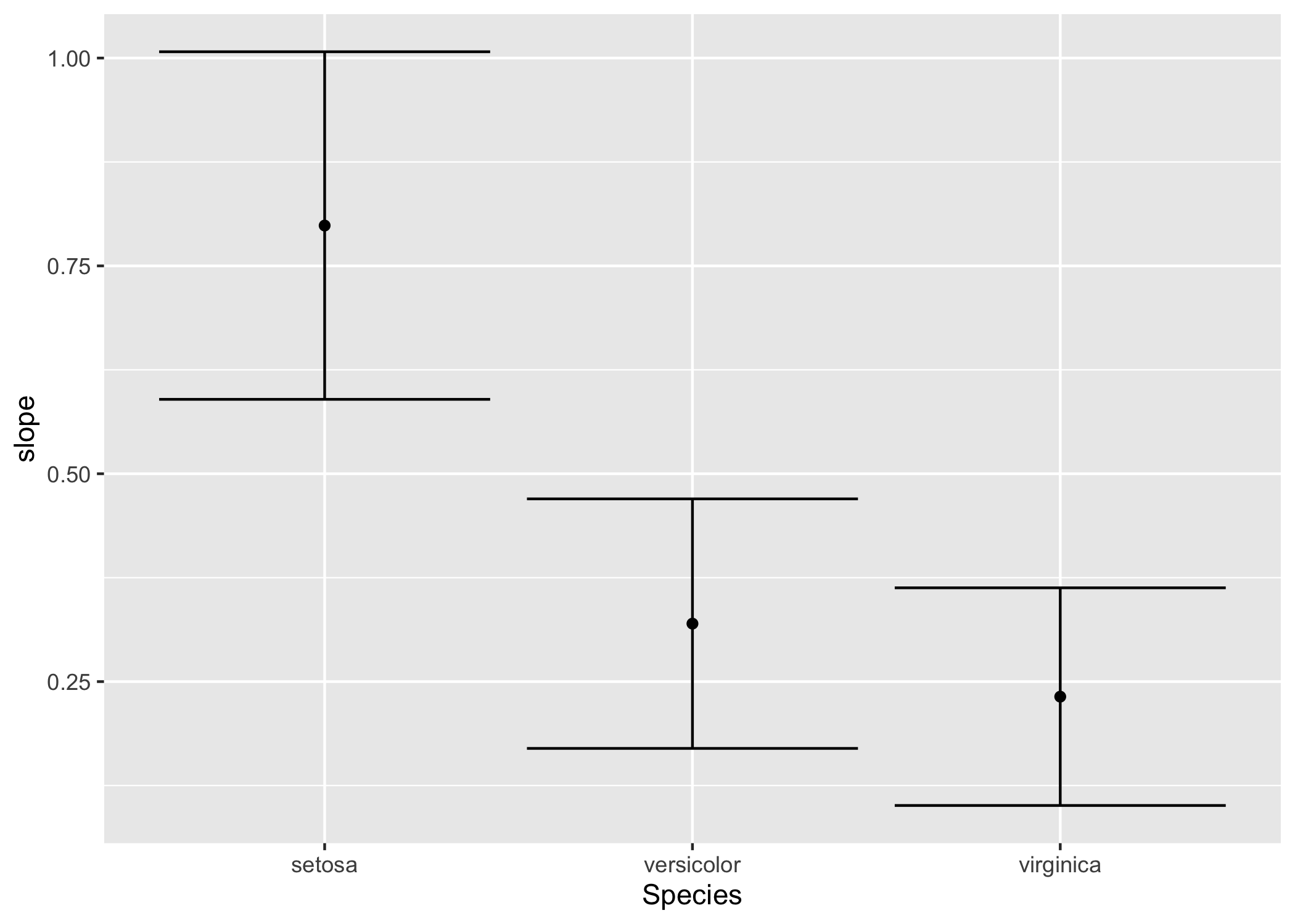
Note that this final result only computed each model once, only computed the confindence intervals once, and managed to make the output figure without once creating an intermediate object!